The Internet’s viral sensation of August 2014 was an off-menu Arby’s sandwich known as the “Meat Mountain." For the low, low price of $10 you can get a stack of eight meats and two cheeses. I think even PETA has been too shocked to respond. And what exactly does this have to do with Microsoft Excel? I’m going to help you use two worksheet cells to create a clickable link to your nearest purveyor of said Meat Mountain. I’ll then show you how to create clickable links to more relevant information, such as property tax bills, or specific locations within a workbook.
Our quest for the 1,275 calorie Meat Mountain begins at Arby’s Locations page, where you’ll enter your ZIP code. In my case, I’m 1.6 miles away from shaving a couple years off of my life if I choose to, but I’ll let this dude serve as my proxy instead. Back to our quest, notice in Figure 1 the ZIP code that I searched for appears in the browser address bar. This means I can use the HYPERLINK function in Excel to create a clickable link to launch the Arby’s web page that will perform a search for any ZIP code I choose.
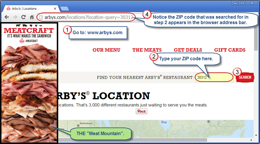
Figure 1: The ZIP code in the browser address bar will help us create a clickable link in Excel using the HYPERLINK function.
The HYPERLINK function in Excel has two arguments:
– link_location – This required argument can be one of many things:
- A web site address
- A cell address or range name within an Excel workbook
- A path and file name of a document on your hard drive
- A bookmark in a Microsoft Word document
The link location can either be enclosed in quotes, or be typed within a worksheet cell and referenced by the cell address.
– friendly_name – This optional argument allows you to specify alternate text instead of the link address. Wrap any text in quotes or refer to a worksheet cell that contains the text you wish to display.
There’s one more mouthful of Excel knowledge we need to swallow in our quest, which is the concept of concatenation. This geeky term translates to stringing pieces of text together, which is what we’ll need to do to dynamically inject our ZIP code of choice into our clickable link. Although Excel does offer a CONCATENATE function, I’m not going to explain it here because you can use the ampersand (&) character instead.
So, off to a blank spreadsheet we go. Type a ZIP code of your choice in cell A1 and then in cell B1 paste the URL from your browser, or type the address shown in step 2 of Figure 1. We’ll make the equivalent of an Excel formula mountain by adding a few layers:
First add an equal sign at the far left of cell B1, and then enclose the existing text in double-quotes, so that the cell contents take this form:
="http://arbys.com/locations?location-query=30312"
Next we need to make the ZIP code portion dynamic, so in my case I’ll replace 30312 with:
"&A1
The revised formula should look like this:
="http://arbys.com/locations?location-query="&A1
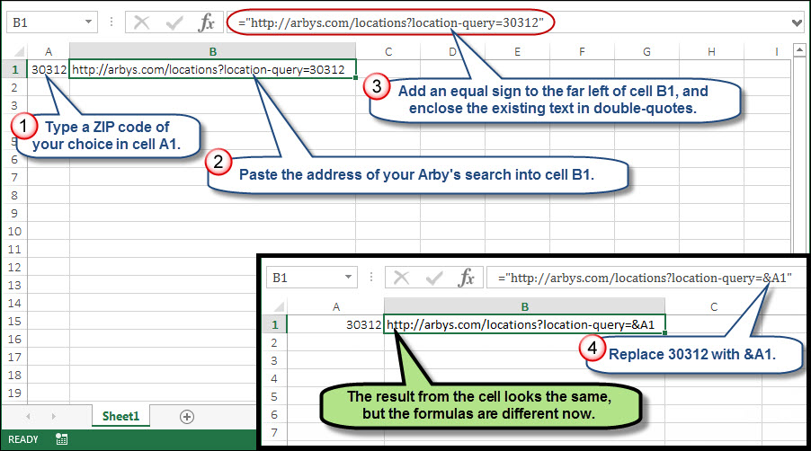
Figure 2: Modify cells A1 and B1 to create a dynamic link to the Arby’s website. At this point the link isn’t clickable.
This gives us the address we’ll need for the web page in question, but to make it clickable we’ll need to add the HYPERLINK function, as shown here:
=HYPERLINK("http://arbys.com/locations?location-query="&A1,"MM")
Feel free to replace "MM" with "Heigh-Ho, heigh-ho, it’s off to Meat Mountain we go" if you choose.
You can now change out the ZIP code in cell A1 as needed to determine the closest Meat Mountain to your house, your office, your gym, or perhaps your primary care physician.

Figure 3: Use the HYPERLINK function to help navigate you to the nearest Arby’s from which you can indulge in the delectable Meat Mountain.
Continuing with our Arby’s theme, let’s see how to use the HYPERLINK function to look up the property tax bills from the last three years for an Atlanta area Arby’s location. This is public information that I was able to look up courtesy of my county tax assessor’s web site. I’ve listed the Parcel ID in cell B1, as illustrated in Figure 4.
Parcel ID: 14 -0130-0010-054-9
In cells A2 through A4, enter the years you would like to see the tax bills for. In this example I entered 2012, 2013 and 2014. Next, in cell B2 enter this URL:
www.fultoncountytaxes.org/property-taxes/TaxBill/Detail?ParcelID=06%20-0368-%20%20LL-149-9&Year=2012
In this case we’ll replace the Parcel ID with a reference to an adjacent worksheet cell:
="https://www.fultoncountytaxes.org/property-taxes/TaxBill/Detail?ParcelID="&$B$1&"&Year=2012"
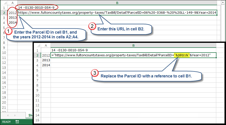
Figure 4: Replace the parcel ID with a reference to cell B1.
One caveat here is that some of this parcel ID contains a space, which web browsers refer to as %20. A quick addition of the SUBSTITUTE function will do the trick:
="https://www.fultoncountytaxes.org/property-taxes/TaxBill/Detail?ParcelID="&SUBSTITUTE($B$1," ","%20")&"&Year=2012"
We then wrap that in the HYPERLINK function:
=HYPERLINK("https://www.fultoncountytaxes.org/property-taxes/TaxBill/Detail?ParcelID="&SUBSTITUTE($B$1," ","%20")&"&Year=2012","2012 Tax Bill")
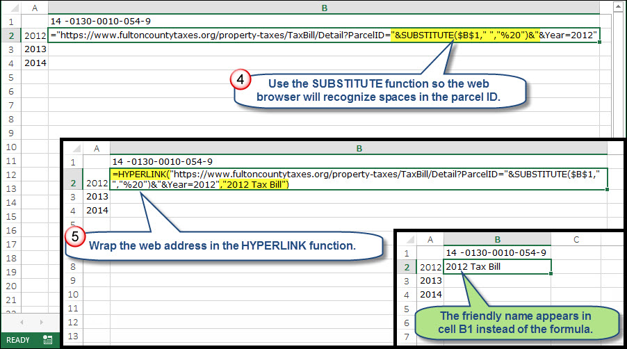
Figure 5: Use the SUBSTITUTE function to enable the web browser to recognize spaces in the parcel ID. Then, wrap your address with the HYPERLINK function.
One last tweak will make the year be dynamic as well:
=HYPERLINK("https://www.fultoncountytaxes.org/property-taxes/TaxBill/Detail?ParcelID="&SUBSTITUTE($B$1," ","%20")&"&Year="&A2,A2&" Tax Bill")
You can now copy this down through cells A3 and A4 and all 3 links will be clickable. Change the Parcel ID in cell B1, and you’ll have one click access to tax bills for the Arby’s location of your choice.
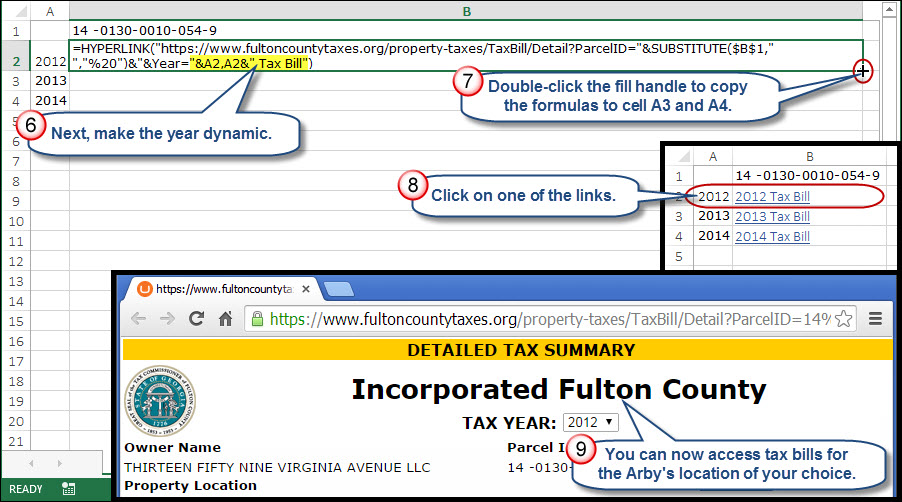
Figure 6: The HYPERLINK function can now look-up tax bills for various years. Change the parcel ID in cell B1 to view the tax bills for a different location.
I will say that recreating Internet addresses can be painstaking work, so do pay attention to details, and build the formula one step at a time as I’ve shown here. You can use this technique with any website that displays your search term in the address bar, so you could build a ZIP code search for McDonald’s in Excel, but not Chipotle or the black cheeseburger offered by Burger King in Japan.
Moving a little farther afield, you can initiate Google searches from Excel as well:
Enter the words “bypass surgery” in cell A1 of a blank worksheet
Enter this formula in cell B1:
=HYPERLINK("https://www.google.com/#q="&SUBSTITUTE(A1," ","+"),"Google Search")
As you can see, Google searches require a + sign instead of %20.
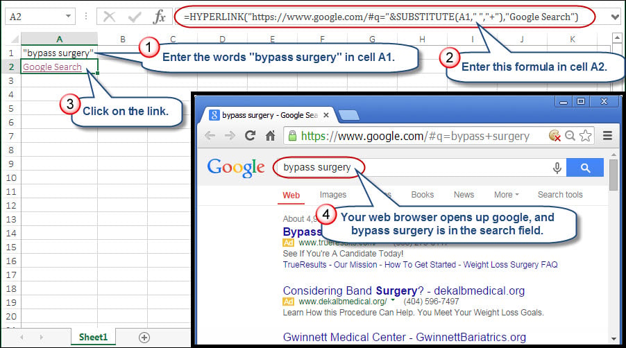
Figure 7: Use the HYPERLINK function to initiate Google searches from Excel.
Now that we’ve covered Internet searches ad nauseam (for that matter, just the thought of a Meat Mountain brings me to the edge of hurling), I’ll close with a more mundane use of the HYPERLINK function. Let’s say that you want a clickable link to any location within a workbook, such as cell A1 of Sheet1 of Book1. In this case your context will be:
=HYPERLINK("[Book1.xlsx]Sheet1!A1","Cell A1 of Sheet1")
Note that for the HYPERLINK function to work you must include the workbook name in square brackets, and separate the sheet name from the cell reference with an exclamation point.
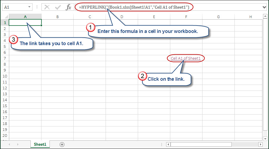
Figure 8: Use the HYPERLINK function to link to a specific location within a workbook.
And that's it. Now either you're starving or need a shot of Pepto.
About the author:
David H. Ringstrom, CPA, heads up Accounting Advisors, Inc., an Atlanta-based software and database consulting firm providing training and consulting services nationwide. Contact David at david@acctadv.com or follow him on Twitter. David speaks at conferences about Microsoft Excel, teaches webcasts for CPE Link, and writes freelance articles on Excel for AccountingWEB, Going Concern, et.al.